A Deterministic View of Diffusion Models
In this post, we present a deterministic perspective on diffusion models. In this approach, neural networks are trained as an inverse function of the deterministic diffusion mapping that progressively corrupts images at each timestep. This method simplifies the derivation of diffusion models, making the process more straightforward and comprehensive.
In recent years, diffusion models, a novel category of deep generative models $[1]$, have made significant strides in producing high-quality, high-resolution images. Notable examples include GLIDE $[2]$, DALLE-2 $[3]$, Imagen, and the fully open-source Stable Diffusion. These models are traditionally built on the framework of Denoising Diffusion Probabilistic Models (DDPM) $[4]$. In this probabilistic framework, the forward diffusion process is modeled as a Gaussian process with Markovian properties. Conversely, the backward denoising process employs neural networks to estimate the conditional distribution at each timestep. The neural networks involved in the denoising process are trained to minimize the evidence lower bound (ELBO) $[4]$ $[5]$, akin to the approach used in a Variational Autoencoder (VAE).
In this post, we present a deterministic perspective on diffusion models. In this method, neural networks are constructed to function in the opposite way of a deterministic diffusion process that gradually deteriorates images over time. This training allows the neural networks to reconstruct or generate images by reversing the diffusion process. This method simplifies the derivation of diffusion models, making the process more straightforward and comprehensive.
Forward Diffusion Process
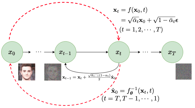
As shown in Figure 1, starting with any input image, denoted as $\mathbf{x}_0$, drawn from a data distribution $p(\mathbf{x})$, the forward process incrementally corrupts the input image for each time step $t=1,2,\cdots,T$. This corruption is achieved by progressively adding varying levels of Gaussian noises as
\[\mathbf{x}_t = \sqrt{\alpha_t } \mathbf{x}_{t-1} + \sqrt{1- \alpha_t } \, {\boldsymbol \epsilon}_t \;\;\;\;\;\; \forall t=1, 2, \cdots, T\]adhering to a predefined noise schedule: $\alpha_1, \alpha_2, \ldots, \alpha_T$, where the noise at each timestep is Gaussian, ${\boldsymbol \epsilon}_t \sim \mathcal{N}(0, \mathbf{I})$. This process gradually introduces more noise at each step, leading to a sequence of increasingly corrupted versions of the original image: $\mathbf{x}_0 \to \mathbf{x}_1 \to \mathbf{x}_2 \to \cdots \to \mathbf{x}_T$. When $T$ is large enough, the last image $\mathbf{x}_T$ approaches to a Gaussian noise, i.e. $\mathbf{x}_T \sim \mathcal{N}(0, \mathbf{I})$.
Building on the so-called “nice property” outlined in $[4]$ $[5]$ $[6]$, the above diffusion process can be implemented much more efficiently. Rather than sampling a unique Gaussian noise at each timestep, it is feasible to sample a single Gaussian noise, $ \boldsymbol{\epsilon} \sim \mathcal{N}(0, \mathbf{I})$, and employ the subsequent formula to efficiently generate all the corrupted samples in one go (along the left-to-right red dash arrow in Figure 1):
\[\mathbf{x}_t = f(\mathbf{x}_{0},t) = \sqrt{\bar{\alpha}_t} \mathbf{x}_{0} + \sqrt{1 - \bar{\alpha}_t} \, {\boldsymbol \epsilon} \;\;\;\;\;\; \forall t=1, 2, \cdots, T\]where
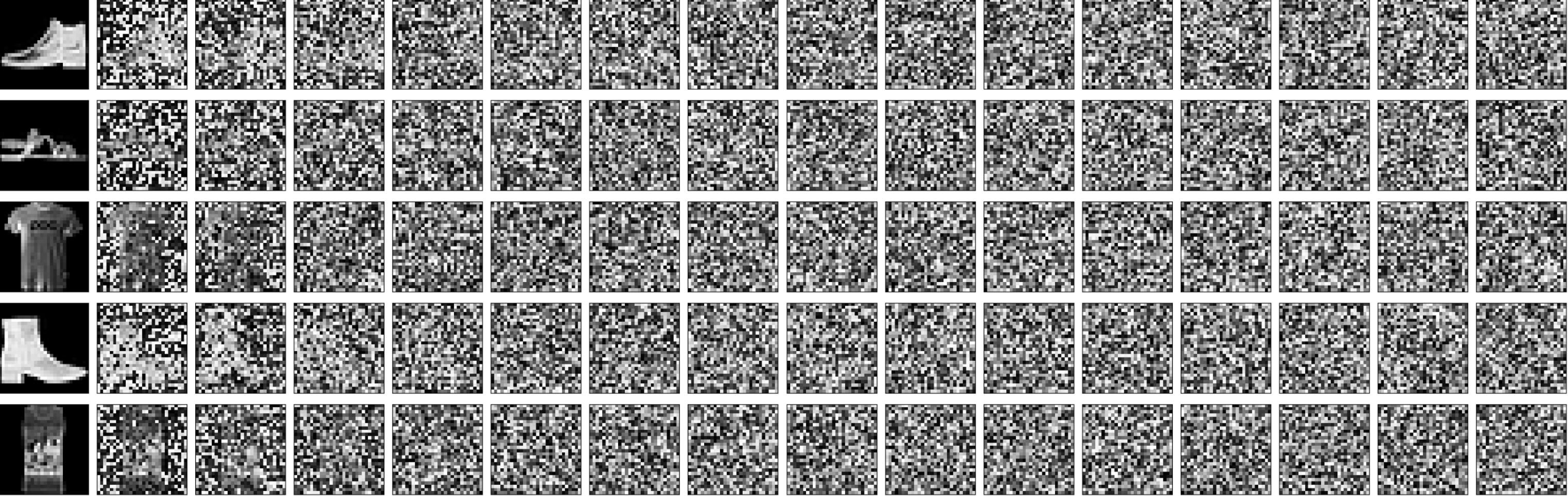
\[\bar{\alpha}_t = \prod_{s=1}^t \alpha_s\]and we have $\bar{\alpha}_t \to 0$ as $t \to T$. As shown in Figure 2, clean images are gradually converted into pure noises in the above deterministic diffusion process as $t$ goes from $0$ to $T$. This method streamlines the process, making the generation of corrupted samples more straightforward and less computationally demanding.
Assuming the application of the aforementioned formula in the diffusion process, let’s explore the relationship between between $\mathbf{x}_{t-1}$ and $\mathbf{x}_t$ in this case. This exploration will help us understand how consecutive stages in the diffusion process are interrelated, which is crucial in the subsequent backward denoising process. In fact, it’s possible to establish how these two consecutive samples are connected using two distinct approaches.
First of all, we have
\[\mathbf{x}_0 = \frac{1}{\sqrt{\bar{\alpha}_t}} \big[ \mathbf{x}_t - \sqrt{1 - \bar{\alpha}_t}\, {\boldsymbol \epsilon} \big]\]and substitue the above to further derive the relationship between any two adjacent samples as follows:
\[\begin{aligned} \mathbf{x}_{t-1} &= \sqrt{\bar{\alpha}_{t-1}} \mathbf{x}_{0} + \sqrt{1 - \bar{\alpha}_{t-1}} \, {\boldsymbol \epsilon} \\ &= \frac{1}{\sqrt{\alpha_t}} \big[ \mathbf{x}_t - \sqrt{1 - \bar{\alpha}_t}\, {\boldsymbol \epsilon} \big] + \sqrt{1 - \bar{\alpha}_{t-1}} \, {\boldsymbol \epsilon} \\ &= \frac{1}{\sqrt{\alpha_t}} \Big[ \mathbf{x}_t - \big( \sqrt{1-\bar{\alpha}_t} - \sqrt{\alpha_t-\bar{\alpha}_t} \big) {\boldsymbol \epsilon} \Big] \\ &= \frac{1}{\sqrt{\alpha_t}} \Big[ \mathbf{x}_t - \frac{1-\alpha_t}{\sqrt{1-\bar{\alpha}_t} + \sqrt{\alpha_t-\bar{\alpha}_t}}\, {\boldsymbol \epsilon} \Big] \\ &\approx \begin{cases} \frac{1}{\sqrt{\alpha_t}} \big[ \mathbf{x}_t - \frac{1-\sqrt{\alpha_t}}{\sqrt{1-\bar{\alpha}_t}}\, {\boldsymbol \epsilon} \big] & \;\;(\mathrm{as} \; \bar{\alpha}_t \approx \bar{\alpha}_{t-1}) \\ \frac{1}{\sqrt{\alpha_t}} \Big[ \mathbf{x}_t - \frac{1-\alpha_t}{2\sqrt{1-\bar{\alpha}_t}}\, {\boldsymbol \epsilon} \Big] & \;\;(\mathrm{as} \; \alpha_t \approx 1) \end{cases} \end{aligned}\]Alternatively, we can have
\[{\boldsymbol \epsilon} = \frac{1}{\sqrt{1 - \bar{\alpha}_{t}}} \big[ \mathbf{x}_t - \sqrt{\bar{\alpha}_t} \mathbf{x}_{0}\big]\]and substitute ${\boldsymbol \epsilon}$ into how $\mathbf{x}_{t-1}$ is computed, we have
\[\begin{aligned} \mathbf{x}_{t-1} &= \sqrt{\bar{\alpha}_{t-1}} \mathbf{x}_{0} + \sqrt{1 - \bar{\alpha}_{t-1}} \, {\boldsymbol \epsilon} \\ &= \sqrt{\bar{\alpha}_{t-1}} \mathbf{x}_{0} + \frac{\sqrt{1 - \bar{\alpha}_{t-1}}}{\sqrt{1 - \bar{\alpha}_{t}}} \big[ \mathbf{x}_t - \sqrt{\bar{\alpha}_t} \mathbf{x}_{0}\big] \\ \end{aligned}\]If we denote
\[\bar{\gamma}_t = \frac{1-\bar{\alpha}_{t-1}}{1-\bar{\alpha}_{t}}\]we can simplify the above equation as follows:
\[\begin{aligned} \mathbf{x}_{t-1} &= \sqrt{\bar{\gamma}_t} \, \mathbf{x}_t + \big( \sqrt{\bar{\alpha}_{t-1}} - \sqrt{\bar{\gamma}_t \bar{\alpha}_t} \big) \mathbf{x}_0 \\ &= \sqrt{\bar{\gamma}_t} \, \mathbf{x}_t + \frac{\bar{\alpha}_{t-1} (1 - \bar{\gamma}_t \alpha_t)}{\sqrt{\bar{\alpha}_{t-1}} + \sqrt{\bar{\gamma}_t \bar{\alpha}_t} }\mathbf{x}_0 \\ &\approx \sqrt{\bar{\gamma}_t} \, \mathbf{x}_t + \frac{\sqrt{\bar{\alpha}_{t-1}} (1 - \bar{\gamma}_t \alpha_t)}{2}\mathbf{x}_0 \;\;\;\;\;\;\;\;(\mathrm{as} \; \bar{\gamma}_t \approx 1 \;\mathrm{and} \; \bar{\alpha}_{t} \approx \bar{\alpha}_{t-1}) \end{aligned}\]Backward Denoising Process
In the backward process, starting from a Gaussian noise
\[\mathbf{x}_T \sim \mathcal{N}(0, \mathbf{I})\]we gradually recover all corrupted images backwards one by one until we obtain the initial clean image:
\[\mathbf{x}_T \to \mathbf{x}_{T-1} \to \mathbf{x}_{T-2} \to \cdots \to \mathbf{x}_1 \to \mathbf{x}_0\]Alternatively, at each timestep, given the corrupted image $x_t$, we may also directly estimate the original clean image $x_0$ based on $x_t$. If the estimate is good enough, we can terminate the above backward denoising process at an earlier stage; Otherwise, we further denoise one timestep backwards, i.e. deriving $x_{t-1}$ from $x_t$. Based on $x_{t-1}$, we may derive a better estimate of the clean image $x_0$. This sampling process continues until we finally obtain a sufficiently good clean image $x_0$.
In order to recover a slightly cleaner version of the image $x_{t-1}$ from $x_{t}$, we have two choices:
I. Estimating clean image $\mathbf{x}_0$
In this case, we construct a deep neural network $\boldsymbol \theta$ to approximate the inverse function of the above diffusion mapping $\mathbf{x}_t = f(\mathbf{x}_0, t)$, denoted as
\[\mathbf{\hat x}_0 = f^{-1}_{\boldsymbol \theta} (\mathbf{x}_t, t)\]which can recover a rough estimate of the clean image $\hat{\mathbf{x}}_0$ from $\mathbf{x}_t$ (along the right-to-left red dash arrow in Figure 1). In this case, this neural network is learned by minimizing the following objective function:
\[\begin{aligned} L_1({\boldsymbol \theta}) &= \sum_{\mathbf{x}_0} \sum_{t=1}^T \Big( f^{-1}_{\boldsymbol \theta} (\mathbf{x}_t, t) - \mathbf{x}_0\Big)^2 \\ &= \sum_{\mathbf{x}_0} \sum_{t=1}^T \Big( f^{-1}_{\boldsymbol \theta} \big(\sqrt{\bar{\alpha}_t} \mathbf{x}_{0} + \sqrt{1 - \bar{\alpha}_t} \, {\boldsymbol \epsilon}, t \big) - \mathbf{x}_0\Big)^2 \end{aligned}\]Once we have learned this neural network, we can derive:
\[\begin{aligned} \mathbf{x}_{t-1} &= \sqrt{\bar{\gamma}_t} \, \mathbf{x}_t + \big( \sqrt{\bar{\alpha}_{t-1}} - \sqrt{\bar{\gamma}_t \bar{\alpha}_t} \big) \hat{\mathbf{x}}_0 % \mathbf{x}_t + \frac{\sqrt{\bar{\alpha}_{t-1}} (1- \alpha_t)}{2} \\ &= \sqrt{\bar{\gamma}_t} \, \mathbf{x}_t + \big( \sqrt{\bar{\alpha}_{t-1}} - \sqrt{\bar{\gamma}_t \bar{\alpha}_t} \big) f^{-1}_{\boldsymbol \theta} (\mathbf{x}_t, t) \end{aligned}\]At last, the sampling process to generate a new image can be described as follows:
- sample a Gaussian noise $\mathbf{x}_T \sim \mathcal{N}(0, \mathbf{I}) $
- for $t=T, T-1, \cdots, 1$:
- compute
- if $\hat{\mathbf{x}}_0$ is stable, return $\hat{\mathbf{x}}_0$
- else denoise one step backward as
- return $\mathbf{x}_0$
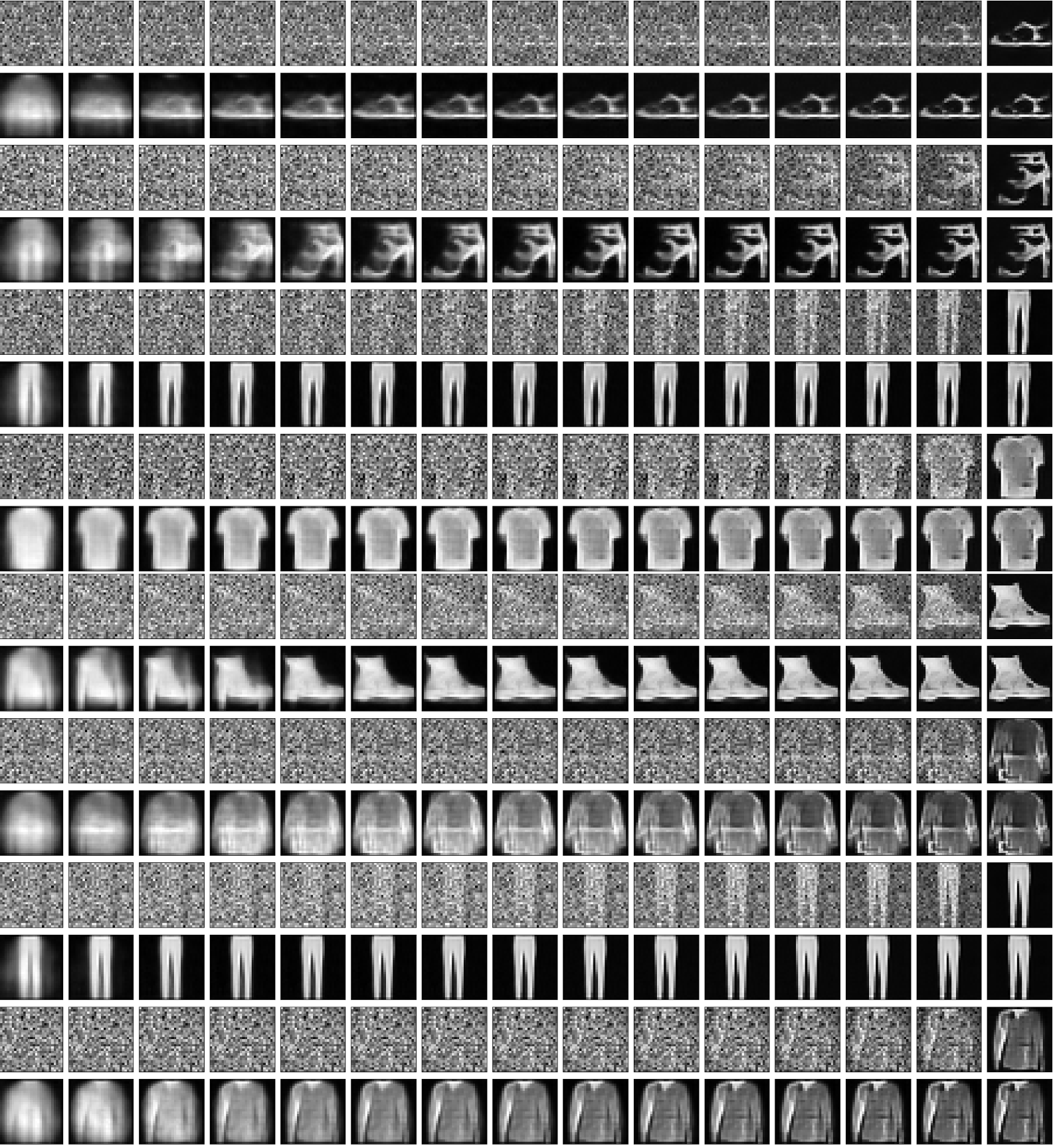
In Figure 3, we have shown some sampling results from the MNIST-Fashion dataset via building neural networks to estimate clean images through the above sampling algorithm.
II. Estimating noise ${\boldsymbol \epsilon}$
In this case, we construct a deep neural network $\boldsymbol \theta$ to approximate the inverse function via estimating the noise ${\boldsymbol \epsilon}$ from each corrupted image $\mathbf{x}_t$ at each timestep $t$:
\[\hat{\boldsymbol \epsilon} = g^{-1}_{\boldsymbol \theta} (\mathbf{x}_t, t)\]This neural network is learned by minimizing the following objective function:
\[\begin{aligned} L_2({\boldsymbol \theta}) &= \sum_{\mathbf{x}_0} \sum_{t=1}^T \Big( g^{-1}_{\boldsymbol \theta} (\mathbf{x}_t, t) - {\boldsymbol \epsilon}\Big)^2 \\ &= \sum_{\mathbf{x}_0} \sum_{t=1}^T \Big( g^{-1}_{\boldsymbol \theta} \big(\sqrt{\bar{\alpha}_t} \mathbf{x}_{0} + \sqrt{1 - \bar{\alpha}_t} \, {\boldsymbol \epsilon}, t \big) - {\boldsymbol \epsilon}\Big)^2 \end{aligned}\]Once we have learned this neural network, we can derive an estimate of $\mathbf{x}_{t-1}$ as follows:
\[\begin{aligned} \mathbf{x}_{t-1} &= \frac{1}{\sqrt{\alpha_t}} \Big[ \mathbf{x}_t - \frac{1-\sqrt{\alpha_t}}{\sqrt{1-\bar{\alpha}_t}}\, \hat{\boldsymbol \epsilon} \Big] \\ &= \frac{1}{\sqrt{\alpha_t}} \Big[ \mathbf{x}_t - \frac{1-\sqrt{\alpha_t}}{\sqrt{1-\bar{\alpha}_t}}\, g^{-1}_{\boldsymbol \theta} (\mathbf{x}_t, t) \Big] \end{aligned}\]At last, the sampling process to generate a new image can be described as follows:
-
sample a Gaussian noise $\mathbf{x}_T \sim \mathcal{N}(0, \mathbf{I}) $
-
for $t=T, T-1, \cdots, 1$:
-
compute $\hat{\boldsymbol \epsilon} = g^{-1}_{\boldsymbol \theta} (\mathbf{x}_t, t)$ and $\hat{\mathbf{x}}_0 = \frac{1}{\sqrt{\bar{\alpha}_t}} \big[ \mathbf{x}_t - \sqrt{1 - \bar{\alpha}_t}\,
\hat{\boldsymbol \epsilon} \big]$ -
if $\hat{\mathbf{x}}_0$ is stable, return $\hat{\mathbf{x}}_0$
-
else denoise one step backward as
-
- return $\mathbf{x}_0$
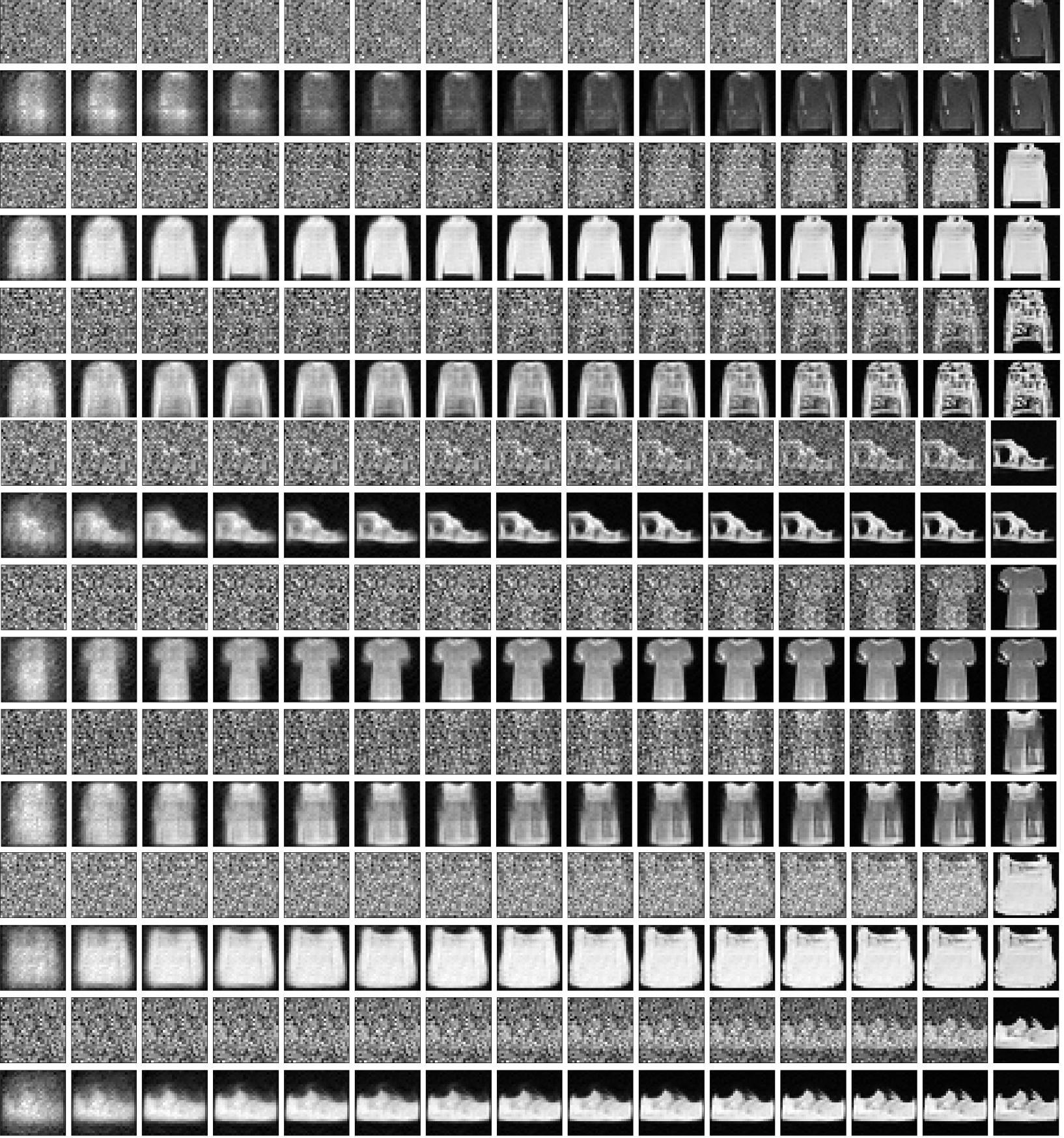
In Figure 4, we have shown some sampling results from the MNIST-Fashion dataset via building neural networks to estimate noises through the above sampling algorithm.
The above two methods are equivalent to the so-called Denoising Diffusion Implicit Models (DDIMs) method referenced in [7]. However, they are derived from a simpler and more intuitive procedure than the one described in [7].
References
$[1]$ Hui Jiang, Machine Learning Fundamentals, Cambridge University Press, 2021.
$[2]$ Alex Nichol, Prafulla Dhariwal, et.al., GLIDE: Towards Photorealistic Image Generation and Editing with Text-Guided Diffusion Models, arXiv:2112.10741 , 2021.
$[3]$ Aditya Ramesh, Prafulla Dhariwal, et.al., Hierarchical Text-Conditional Image Generation with CLIP Latents, arXiv:2204.06125 , 2022.
$[4]$ Jonathan Ho, Ajay Jain, Pieter Abbeel, Denoising Diffusion Probabilistic Models, arXiv:2006.11239 , 2020.
$[5]$ Calvin Luo, Understanding Diffusion Models: A Unified Perspective, arXiv:2208.11970 , 2022.
$[6]$ Sergios Karagiannakos,Nikolas Adaloglou, How diffusion models work: the math from scratch, https://theaisummer.com/diffusion-models/.
$[7]$ Jiaming Song, Chenlin Meng, Stefano Ermon, Denoising Diffusion Implicit Models, arXiv:2010.02502, 2020.