An Introduction to Zero-Knowledge Proofs and zk-SNARKs
This post introduces zero-knowledge proofs and explains how zk-SNARKs allow a prover to convince a verifier that a computation is correct without revealing private inputs. It develops the full path from arithmetic circuits to R1CS and QAPs with concrete examples, then shows how elliptic curves, bilinear pairings, and Groth16 turn these algebraic ideas into practical zero-knowledge proofs.
Abstract
This tutorial introduces zero-knowledge proofs and explains how zk-SNARKs let a prover convince a verifier that a computation is correct without revealing the private inputs. It develops the full algebraic pipeline from arithmetic circuits to R1CS, then from R1CS to Quadratic Arithmetic Programs (QAPs), using concrete examples to make the constructions intuitive. The paper also explains why elliptic-curve commitments and bilinear pairings are needed to turn polynomial satisfaction into an efficient zero-knowledge proof. Finally, it presents Groth16 in detail, highlighting its main components, proof flow, and practical significance.
1. Introduction
What is a zero-knowledge proof?
A zero-knowledge proof (ZKP) is a protocol that lets a prover convince a verifier that a statement is true without revealing the witness that makes the statement true.
Typical examples of statements are:
- “I know a password that hashes to this public digest.”
- “I know a valid solution to this Sudoku puzzle.”
- “This private transaction conserves value and uses authorized inputs.”
- “I executed this computation correctly.”
The central idea is subtle but powerful: instead of revealing the secret, the prover demonstrates possession of the secret in a mathematically checkable way.
Why are zero-knowledge proofs needed?
Modern digital systems often require two things at the same time:
- correctness: the verifier wants assurance that a computation or claim is valid;
- privacy: the prover does not want to disclose sensitive inputs.
Without ZKPs, systems often fall into one of two bad extremes:
- reveal everything so correctness can be checked; or
- hide everything and ask others to trust you.
Zero-knowledge proofs provide a third option: prove correctness without revealing the hidden data.
This is useful in many settings:
- Privacy-preserving payments: prove that a transaction is well formed, authorized, and value-conserving without revealing sender/receiver/value details.
- Verifiable computation: a server proves it executed a program correctly on private or large inputs.
- Rollups and blockchain scaling: many off-chain transactions are compressed into one succinct proof checked on-chain.
- Private voting and auctions: prove validity of ballots or bids without exposing them.
From general ZKPs to zk-SNARKs
A zk-SNARK is a special kind of zero-knowledge proof system:
- zk = zero knowledge;
- S = succinct (proofs are small and verification is fast);
- N = non-interactive (the prover sends one proof message instead of a back-and-forth dialogue);
- AR = argument (security may rely on computational assumptions rather than information-theoretic guarantees);
- K = knowledge (the prover is proving knowledge of a witness).
Informally, a zk-SNARK lets you prove:
“I know private inputs
wsuch that a public computationC(x, w)outputs1.”
Here:
-
xis the public input; -
wis the private witness; -
Cis a program or circuit; - output
1means the statement is satisfied.
The power of zk-SNARKs comes from a compilation pipeline:
program -> arithmetic circuit -> R1CS -> QAP -> cryptographic proof
This tutorial follows exactly that pipeline.
What makes zk-SNARKs special?
Compared with a generic proof system, zk-SNARKs are attractive because they often have:
- very small proofs;
- fast verification;
- support for complex computations;
- strong privacy guarantees.
The tradeoff is that classical pairing-based zk-SNARKs such as Groth16 require a trusted setup tailored to the circuit.
A concrete mental model
Suppose Alice wants to prove to Bob that she knows secret values x, y, and z such that
x * y + z = 35
without revealing x, y, or z.
For example, Alice may know:
x = 3, y = 10, z = 5
since 3 * 10 + 5 = 35.
A zk-SNARK will let Alice prove the truth of the statement
There exist x, y, z such that x*y + z = 35.
without revealing the witness (x, y, z).
The rest of the tutorial explains how such a statement is transformed into algebraic objects that can be proved efficiently.
2. Algebraic Circuits
Why arithmetic circuits?
To build a zk-SNARK, we first need a representation of computation that is friendly to algebra. Ordinary programs have branches, loops, memory, and machine instructions. zk-SNARKs instead work naturally with arithmetic circuits over a finite field F.
An arithmetic circuit is a directed acyclic graph whose gates perform field operations such as:
- addition;
- multiplication;
- multiplication by constants.
Boolean logic can be encoded too, but the native language is arithmetic.
Example: a tiny arithmetic circuit
Let us encode the statement
x * y + z = out
with public output out = 35 and private witness (x, y, z).
A simple circuit is:
t1 = x * y
t2 = t1 + z
assert t2 = out
A circuit diagram is:
x ----\
       (*) ---- t1 ---\
y ----/                (+) ---- t2 ---- [assert equals out]
                      /
z -------------------/
This circuit has:
- one multiplication gate;
- one addition gate;
- one equality check.
Another example: proving u >= v
In this example, we demonstrate how to use equality constraints to prove inequality relation u >= v. We constrain u and v to be at most n-1 bit numbers. We create an arithmetic circuit that encodes the binary represetation of 2^{n-1} + (u - v) using n bits. If the most significant bit of 2^{n-1} + (u - v) is 1, then u >= v and vice versa.
Here we assume n=4 for simplicity. The final arithmetic circuit to check u >= v is given as follows.
// u and v are represented with at most 3 bits:
2^2 * a2 + 2^1 * a1 + a0 == u
2^2 * b2 + 2^1 * b1 + b0 == v

// binary constraints (0 or 1) for ai, bi
a0 * (a0 - 1) == 0
a1 * (a1 - 1) == 0
a2 * (a2 - 1) == 0
b0 * (b0 - 1) == 0
b1 * (b1 - 1) == 0
b2 * (b2 - 1) == 0

// 2n−1 + (x - y) binary representation
2^3 + (u - v) == 8 * c3 + 4 * c2 + 2 * c1 + c0

// binary constraints (0 or 1) for ci
c0 * (c0 - 1) == 0
c1 * (c1 - 1) == 0
c2 * (c2 − 1) == 0
c3 * (c3 − 1) == 0

// Check that the MSB is 1
assert c3 === 1
Wires, assignments, and constraints
A circuit is evaluated by assigning values to all its wires. For the first example:
x = 3
y = 10
z = 5
t1 = 30
t2 = 35
out = 35
The witness usually includes all private values and intermediate wire values needed to satisfy the circuit. In this case, the witness is
w = [x, y, z, t1, t2] = [3, 10, 5, 30, 35]
and the public input is
i = [out] = [35]
A zk-SNARK prover does not just prove the final result. It proves that every gate is locally consistent with one global assignment of all wires using the private witness and the public input.
Turning circuits into R1CS
The standard next step is to convert the circuit into a Rank-1 Constraint System (R1CS).
An R1CS instance is a list of constraints of the form
\[\langle A_i, s \rangle \times \langle B_i, s \rangle = \langle C_i, s \rangle\]where:
-
sis the vector of all variables (both witness and input) assigned to all wires; -
A_i, B_i, C_iare coefficient vectors; -
<., .>is an inner product.
Each constraint includes:
- use
A_ito form one linear combination of variables; - use
B_ito form another linear combination; - multiply them;
- require the result to equal a third linear combination by
C_i.
This form is perfect for multiplication gates, and additions can be implemented as multiplication by embedding an extra 1 in s.
Example: variable vector for x*y + z = out
Let the assignment vector be
s = [1, out, x, y, z, t1, t2]
The leading 1 is a constant wire, which lets us express affine terms like z + out = 10 as (z + out) x 1 = 10.
From the witness and input
out = 35, x = 3, y = 10, z = 5, t1 = 30, t2 = 35
we get
s = [1, 35, 3, 10, 5, 30, 35]
R1CS constraints for the example
We encode the three steps:
Constraint 1: t1 = x * y
x * y = t1
So:
-
A_1selectsx -
B_1selectsy -
C_1selectst1
Vectors:
A_1 = [0, 0, 1, 0, 0, 0, 0]
B_1 = [0, 0, 0, 1, 0, 0, 0]
C_1 = [0, 0, 0, 0, 0, 1, 0]
Then:
<A_1, s> = x = 3
<B_1, s> = y = 10
<C_1, s> = t1 = 30
and indeed 3 * 10 = 30.
Constraint 2: t2 = t1 + z
We rewrite addition as:
(t1 + z) * 1 = t2
Vectors:
A_2 = [0, 0, 0, 0, 1, 1, 0]
B_2 = [1, 0, 0, 0, 0, 0, 0]
C_2 = [0, 0, 0, 0, 0, 0, 1]
Then:
<A_2, s> = z + t1 = 5 + 30 = 35
<B_2, s> = 1
<C_2, s> = t2 = 35
so the constraint holds.
Constraint 3: t2 = out
Rewrite as:
t2 * 1 = out
Vectors:
A_3 = [0, 0, 0, 0, 0, 0, 1]
B_3 = [1, 0, 0, 0, 0, 0, 0]
C_3 = [0, 1, 0, 0, 0, 0, 0]
Then:
<A_3, s> = t2 = 35
<B_3, s> = 1
<C_3, s> = out = 35
Again the constraint holds.
Why R1CS matters
R1CS gives us a uniform algebraic view of computation:
- every gate becomes a quadratic constraint;
- the whole program becomes a list of such constraints;
- proving correctness becomes proving all constraints are satisfied simultaneously.
The next step is the key leap in zk-SNARK design: compressing many constraints into a single polynomial identity.
3. Quadratic Arithmetic Programs
From many constraints to one polynomial identity
An R1CS has many equations:
\[\langle A_i, s \rangle \times \langle B_i, s \rangle = \langle C_i, s \rangle \;\;\;\;\;\;\;\text{for} \;\;i=1,2,\cdots,m\]A Quadratic Arithmetic Program (QAP) packages all of them into a polynomial statement.
The idea is elegant:
- each variable in
sgets three families of polynomialsu_j(X), v_j(X), w_j(X)fromA,BandCrespectively; - evaluating at special points
r_1, ..., r_mcorresponds to selecting constraint rows, for convenience, we usually pick row indexes, i.e.r_1=1, ...., r_m=m. - if the assignment satisfies every R1CS constraint, then one polynomial is divisible by a target polynomial
t(X)(to be explained later).
This is the algebraic heart of pairing-based zk-SNARKs.
The interpolation idea
Suppose there are m constraints. Pick
one for each constraint.
For every variable s_j, for the constraint in row i, define polynomials that satisfy:
These polynomials are obtained by Lagrange interpolation. For example, u_j(X) is a polynomial that passes through the following points:
(1, A_1[j]), (2, A_2[j]), (3, A_3[j]), ....
The similar idea applies to v_j(X) and w_j(X).
Then for a particular assignment s = (s_1, ..., s_n), define
At each constraint point r_i = i, these evaluate to:
So if every R1CS constraint holds, then for every i:
See the following figure:
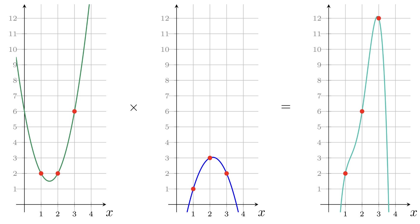
That means the polynomial
\[P(X) = U(X)V(X) - W(X)\]has roots at all points X=1, ..., X=m. See the following figure:
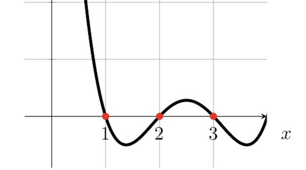
Therefore it must be divisible by
\[t(X) = (X-1)(X-2)...(X-m)\]So there exists a polynomial H(X) such that
This single divisibility statement is equivalent to satisfying all R1CS constraints.
Lagrange interpolation in one line
If a polynomial f(X) must satisfy values f(r_i)=y_i for i=1,...,m, then:
where L_i(X) is the i-th Lagrange basis polynomial:
and it has the property:
\[L_i( r_k ) = \begin{cases} 1 & k = i \\ 0 & k \neq i \end{cases}\]This is exactly what lets us encode each column of the R1CS matrices as polynomials.
A concrete QAP example from the previous R1CS
We continue the first example with three constraints. Pick interpolation points:
\[r_1 = 1, r_2 = 2, r_3 = 3\]Then:
\[t(X) = (X-1)(X-2)(X-3)\]We will derive a few of the QAP polynomials explicitly.
The Lagrange basis polynomials are:
\[L_1(X) = \frac{(X-2)(X-3)}{(1-2)(1-3)} = \frac{1}{2}(X-2)(X-3)\] \[L_2(X) = \frac{(X-1)(X-3)}{(2-1)(2-3)} = -(X-1)(X-3)\] \[L_3(X) = \frac{(X-1)(X-2)}{(3-1)(3-2)} = \frac{1}{2}(X-1)(X-2)\]Example: polynomial for variable x in the A family
Looking at the R1CS rows:
- in constraint 1, coefficient of
xinA_1is1; - in constraint 2, coefficient is
0; - in constraint 3, coefficient is
0.
So u_x(X) must satisfy:
Hence:
\[u_x(X) = L_1(X)\]Example: polynomial for variable y in the B family
Similarly, y appears only in B_1 with coefficient 1, so:
Example: polynomial for t1 in the C family
t1 appears only in C_1, so:
Example: constant wire 1 in the B family
The constant wire appears in:
-
B_1: coefficient0 -
B_2: coefficient1 -
B_3: coefficient1
So:
\[v_1(X) = 0 \times L_1(X) + 1 \times L_2(X) + 1 \times L_3(X) = L_2(X) + L_3(X)\]Building U(X), V(X), W(X)
Given the satisfying assignment
s = [1, 35, 3, 10, 5, 30, 35]
we construct:
\[U(X) = \sum_j s_j u_j(X)\] \[V(X) = \sum_j s_j v_j(X)\] \[W(X) = \sum_j s_j w_j(X)\]We do not need to write every coefficient explicitly to see what happens. By construction:
U(1)=x=3,      V(1)=y=10,      W(1)=t1=30
U(2)=t1+z=35,  V(2)=1,         W(2)=t2=35
U(3)=t2=35,    V(3)=1,         W(3)=out=35
Therefore:
P(1)=U(1)V(1)-W(1)=3*10-30=0
P(2)=35*1-35=0
P(3)=35*1-35=0
So P(X) has roots 1,2,3 and therefore:
meaning P(X) is divisible by t(X).
Why divisibility checks all constraints at once
This is the core compression trick:
- originally, we had three separate R1CS equations;
- after interpolation, we formed one polynomial
P(X); - proving
t(X)dividesP(X)proves all three constraints simultaneously.
For a circuit with millions of constraints, this same logic still holds.
A trusted-setup view of QAP evaluation
Now imagine a setup chooses a secret field element τ, unknown to both prover and verifier after setup.
Instead of revealing the full polynomials, the system can work with their evaluations at the hidden point τ:
If the assignment is valid, then
\[U(\tau)V(\tau) - W(\tau) = H(\tau)t(\tau)\]This is a single field equation at the secret point τ.
Why is this useful?
Because:
- the prover can combine preprocessed setup elements corresponding to
u_j(τ), v_j(τ), w_j(τ); - the verifier only needs to check a compact algebraic relation;
- the hidden evaluation point prevents the prover from faking an invalid polynomial identity by exploiting visible roots.
A concrete symbolic evaluation example
Suppose setup secretly sampled τ = 7. Then the target polynomial is:
t(7) = (7-1)(7-2)(7-3) = 6*5*4 = 120
The prover never learns τ directly, but the proving key contains encodings of values like:
u_j(τ), v_j(τ), w_j(τ)
in cryptographic form.
Using the assignment coefficients s_j, the prover forms encoded versions of:
and also the quotient witness H(τ) satisfying:
At this stage, the math says the witness is valid. But nothing is zero knowledge yet. If we simply revealed these field values, we might leak the witness. The next section explains how cryptography turns this algebraic statement into a true zero-knowledge proof.
4. Zero Knowledge
Why QAP algebra alone is not enough
The QAP statement
\[U(X)V(X)-W(X)=H(X)t(X)\]captures correctness, but not privacy.
If the prover directly sent:
\[U(\tau), V(\tau), W(\tau), H(\tau)\]then those values could leak information about the witness, because each is a linear or nonlinear combination of witness variables.
So the next step is to hide field elements inside cryptographic group elements.
Encoding field elements with elliptic curves
Let G1 and G2 be elliptic curve groups of prime order q, with generators g1 and g2.
A field element a can be encoded as a group element:
This is often called “encoding in the exponent,” even though elliptic-curve groups are written additively.
Why is this useful? Because if discrete logarithms are hard, seeing [a]1 does not reveal a.
At the same time, linear relations are still easy to manipulate:
\[[a]_1 + [b]_1 = [a+b]_1\] \[c * [a]_1 = [ca]_1\]So a prover can build encoded linear combinations of polynomial evaluations without revealing their underlying field values.
Encoding QAP values
During trusted setup, the system can publish encoded basis elements such as:
\[[u_j(\tau)]_1, [v_j(\tau)]_2, [w_j(\tau)]_1\]Then the prover, knowing the witness coefficients s_j, can compute:
without learning τ.
This is already a big step:
- the prover manipulates hidden evaluations algebraically;
- the verifier sees only group elements, not raw field values.
But the verifier still needs a way to check multiplicative relations like
\[U(\tau)V(\tau)\]using only encoded values.
Why bilinear pairings are needed
A bilinear pairing is a map
e: G1 x G2 -> GT
with the crucial property:
\[e([a]_1, [b]_2) = e(g1, g2)^{ab}\]This is exactly what we need: it lets the verifier check multiplicative relations between hidden scalars.
If the prover sends [U(τ)]1 and [V(τ)]2, the verifier can compute:
Similarly, encoded values for W(τ) and H(τ)t(τ) can be combined so that equality of pairings implies the desired polynomial identity.
Conceptual verification equation
At a high level, the verifier wants to check:
\[U(\tau)V(\tau) - W(\tau) = H(\tau)t(\tau)\]In the exponent, this becomes something like:
\[e([U(\tau)]_1, [V(\tau)]_2) = e([W(\tau)]_1 + [H(\tau)t(\tau)]_1, g2)\]This is only a conceptual sketch, not the exact Groth16 equation. The important point is that pairings convert a multiplicative identity over hidden field values into a check over public group elements.
Where zero knowledge comes from
Hiding the witness requires more than just elliptic-curve encodings. Modern zk-SNARKs add random blinding terms.
The prover randomizes proof elements using fresh scalars, often denoted by values like r and s, so that the same witness can generate many unlinkable proofs.
This blinding serves several purposes:
- it hides witness-dependent linear combinations;
- it prevents proof elements from exposing raw QAP evaluations;
So the privacy story is:
- convert computation to algebra;
- evaluate algebra at a hidden setup point;
- encode those evaluations in elliptic-curve groups;
- use randomizers so the encodings reveal nothing about the witness;
- use pairings so the verifier can still check correctness.
5. Groth16 Explained
What is Groth16?
Groth16 is one of the most influential pairing-based zk-SNARK constructions. It is famous because it achieves very small proofs and efficient verification, which is why it has been widely used in practice.
Conceptually, Groth16 takes a circuit compiled into R1CS/QAP form and produces a proof consisting of three group elements:
π = (A, B, C)
The verifier checks a compact pairing equation involving these proof elements, the verification key, and the public inputs.
Inputs to the scheme
Groth16 works with a relation of the form:
R(x, w) = 1
where:
-
x= public inputs; -
w= private witness.
The workflow is:
- Setup: given the circuit, generate a proving key
pkand verifying keyvk. - Prove: using
pk,x, andw, produce proofπ. - Verify: using
vk,x, andπ, accept or reject.
Key ingredients in Groth16
Before stating the algorithm, it helps to name the important ingredients.
(a) The secret evaluation point τ
As in QAPs, Groth16 relies on evaluating polynomials at a hidden point τ chosen during setup.
(b) Additional trapdoors α, β, γ, δ
These extra secret scalars help separate roles in the proof system:
- bind the proof to the correct QAP structure;
- distinguish public-input and private-witness parts;
- enable zero-knowledge randomization.
(c) Public-input separation
Groth16 treats public inputs specially. Part of the verification key contains encoded coefficients used to combine the public inputs into one group element.
This allows the verifier to check the proof against the claimed public instance without learning private witness data.
(d) The quotient polynomial H(X)
Recall:
\[U(X)V(X)-W(X)=H(X)t(X)\]The polynomial H(X) certifies divisibility by the target polynomial. In Groth16, part of the proof encodes information derived from H(τ).
(e) Randomizers r and s
Fresh randomness is used to blind the proof so that it is zero knowledge.
Setup in more detail
Starting from the circuit, compute its QAP description. Then sample secret trapdoors:
τ, α, β, γ, δ
The setup publishes encoded combinations of these values. The exact proving key contains many group elements, but conceptually it includes encodings of:
- polynomial evaluations at
τ; -
α-weighted andβ-weighted variants; - elements divided by
δfor private-witness terms; - target-polynomial-related elements for the quotient witness.
The setup output is:
- proving key
pk: large, used by the prover; - verifying key
vk: small, used by the verifier.
A useful mental picture is:
-
pkis like a cryptographic compiler output for the circuit; -
vkis like a compressed certificate checker.
Groth16 prover structure
Let the full assignment be:
a = (1, x_1, ..., x_l, w_1, ..., w_m)
where the first part corresponds to the public inputs, x_1, ..., x_l, and the second part to private witness variables, w_1, ..., w_m.
The prover forms linear combinations of QAP basis evaluations at τ. Abstractly, it computes hidden values from the secret witness w_1, ..., w_m corresponding to:
and a more complicated third term C combining:
- witness-dependent contributions,
- the quotient witness
H(τ), - zero-knowledge blinding terms.
Then it randomizes them with fresh scalars r and s and outputs three group elements:
A in G1
B in G2
C in G1
A convenient conceptual view is:
A = [A_eval + rδ]1
B = [B_eval + sδ]2
C = [ ... quotient/private terms ... + sA_eval + rB_eval - rsδ ]1
This schematic form is not the full formal equation, but it captures the role of the randomizers and why C must absorb cross terms so the final pairing equation balances.
Verifier structure
The verifier first compresses the public inputs into one group element:
\[P_x = \Big[\gamma_0 + x_1 \gamma_1 + \cdots + x_l \gamma_l \Big]_1\]where the γ_i-related elements come from setup.
Then the verifier checks the core Groth16 pairing equation:
\[e(A, B) = e( [\alpha]_1, [ \beta]_2) + e(P_x, [\gamma]_2) + e(C, [\gamma]_2)\]This is the famous compact check.
Interpretation:
- the left side captures the multiplicative structure of the witness-dependent QAP evaluation;
- the right side reconstructs the expected public-input contribution, fixed setup contribution, and quotient/blinding correction.
If the witness is valid and the proof was formed honestly, the equation holds.
The full Groth16 algorithm and more detailed explanations can be found at an online tutorial.
Why the verifier equation works
At a high level, the pairing equation checks that:
- the witness-dependent linear combinations match the QAP;
- the public inputs are exactly those claimed by the prover;
- the quotient witness accounts for divisibility by
t(X); - the randomizers are incorporated consistently;
- no invalid witness can satisfy the equation except with negligible probability.
The elegance of Groth16 is that all of this collapses into a tiny proof and a tiny verification equation.
Strengths and limitations of Groth16
Strengths
- extremely small proofs;
- very fast verification;
- mature implementations;
- strong fit for blockchains and verifiable computation.
Limitations
- circuit-specific trusted setup;
- prover time and memory can still be large for big circuits;
- less flexible than newer universal-setup systems in some workflows.
Even so, Groth16 remains one of the clearest ways to understand the classical zk-SNARK design pattern.
6. Summary
This tutorial followed the standard pairing-based zk-SNARK pipeline from computation to proof.
We began with the main idea of zero-knowledge proofs: convince a verifier that a statement is true without revealing the witness. This is valuable for privacy-preserving payments, identity systems, blockchain scaling, private voting, and verifiable computation.
We then introduced zk-SNARKs, which make these proofs succinct and non-interactive. The core technical path is:
program -> arithmetic circuit -> R1CS -> QAP -> cryptographic proof
In the algebraic circuit section, we saw how a simple computation such as
x*y + z = out
is broken into gates and then into local algebraic constraints. Those constraints were expressed as R1CS, where each row has the form
\[\langle A_i, s \rangle \times \langle B_i, s \rangle = \langle C_i, s \rangle\]In the QAP section, we used Lagrange interpolation to convert columns of R1CS matrices into polynomials. This turned many individual constraints into one divisibility relation:
\[U(X)V(X)-W(X)=H(X)t(X)\]That identity is the algebraic engine of classical zk-SNARKs.
In the zero-knowledge section, we explained why algebra alone is not enough. To hide the witness while preserving verifiability, the system encodes hidden polynomial evaluations as elliptic-curve group elements and uses bilinear pairings to verify multiplicative relations. Random blinding terms make the resulting proof zero knowledge.
Finally, in Groth16, we saw how this machinery becomes a practical proof system:
- setup generates proving and verifying keys using hidden trapdoors;
- the prover produces a proof
(A, B, C); - the verifier checks a compact pairing equation.
The remarkable result is that a complicated computation can be reduced to a tiny proof that reveals nothing about the witness beyond validity.
Groth16 is not the only zk system, and in modern practice there are many alternatives such as PLONK- and STARK-family systems. But Groth16 remains one of the clearest and most influential examples of how zero-knowledge, algebraic representations of computation, elliptic curves, and pairings come together to form a working zk-SNARK.
References
- Jens Groth, On the Size of Pairing-Based Non-interactive Arguments, EUROCRYPT 2016.
- Vitalik Buterin, Quadratic Arithmetic Programs: from Zero to Hero.
- Zcash Protocol Specification, shielded payments secured by zk-SNARKs.
- Ethereum EIP-196 and EIP-197, elliptic-curve and pairing precompiles used for zk-SNARK verification.
- arkworks
ark-groth16documentation, including R1CS-to-QAP reduction and witness mapping. - Maksym Petus, Why and How zk-SNARK Works, arXiv https://arxiv.org/abs/1906.07221.
- RareSkills Book of Zero Knowledge, https://rareskills.io/zk-book.