A Deterministic View of Diffusion Models
In this post, we present a deterministic perspective on diffusion models. In this approach, neural networks are trained as an inverse function of the deterministic diffusion mapping that progressively corrupts images at each time step. This method simplifies the derivation of diffusion models, enabling us to fully explain and derive them using only a few straightforward mathematical equations.
In recent years, diffusion models, a novel category of deep generative models
In this post, we present a deterministic perspective on diffusion models. In this method, neural networks are constructed to function in the opposite way of a deterministic diffusion process that gradually deteriorates images over time. This training allows the neural networks to reconstruct or generate images by reversing the diffusion process without using any knowledge of stochastic process. This method simplifies the derivation of diffusion models, making the process more straightforward and comprehensible. Within this deterministic framework, diffusion models can be fully explained and derived from scratch using only a few straightforward mathematical equations, as shown in this concise, self-contained post. This approach requires only basic mathematical knowledge, eliminating the need for lengthy tutorials filled with hundreds of complex equations involving stochastic processes and probability distributions.
Deterministic Forward Diffusion Process

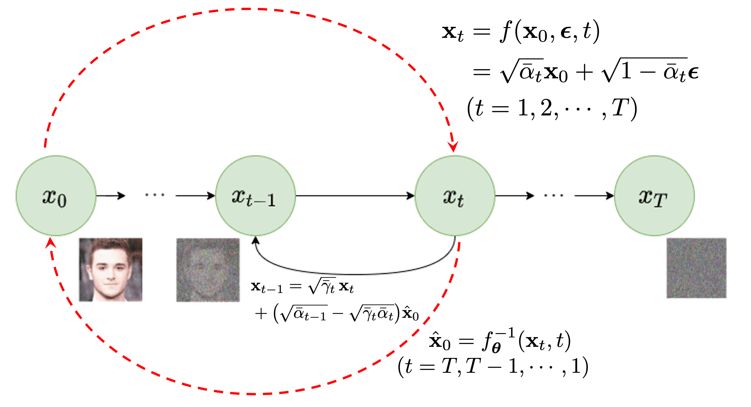
In Figure 1, we illustrate a deterministic view of the typical diffusion process in diffusion models. Starting with any input clean image, denoted as \(\mathbf{x}_0\), the forward process incrementally corrupts the input image for each time step \(t=1,2,\cdots,T\). This corruption is achieved by progressively adding varying levels of Gaussian noises over time as
\[\mathbf{x}_t = \sqrt{\alpha_t } \mathbf{x}_{t-1} + \sqrt{1- \alpha_t } \, {\boldsymbol \epsilon}_t \;\;\; \forall t=1, 2, \cdots, T\]adhering to a predefined noise schedule: \(\alpha_1, \alpha_2, \ldots, \alpha_T\), where the noise at each timestep is Gaussian, \({\boldsymbol \epsilon}_t \sim \mathcal{N}(0, \mathbf{I})\). This process gradually introduces more noise at each step, leading to a sequence of increasingly corrupted versions of the original image: \(\mathbf{x}_0 \to \mathbf{x}_1 \to \mathbf{x}_2 \to \cdots \to \mathbf{x}_T\). When \(T\) is large enough, the last image \(\mathbf{x}_T\) approaches to a Gaussian noise, i.e. \(\mathbf{x}_T \sim \mathcal{N}(0, \mathbf{I})\).
Building on the so-called “nice property” outlined in
where \(\bar{\alpha}_t = \prod_{s=1}^t \alpha_s\) and we have \(\bar{\alpha}_t \to 0\) as \(t \to T\).
In the diffusion process described in Eq. (\ref{eq-forward-deterministic}), once the noise \({\boldsymbol \epsilon}\) is sampled, it is treated as constant for the whole diffusion process. Consequently, the transformation from the clean image \(\mathbf{x}_{0}\) to noisy images \(\mathbf{x}_{t}\) at each time step \(t\) can be regarded as a deterministic mapping, characterized by the above function \(\mathbf{x}_t = f(\mathbf{x}_{0}, {\boldsymbol \epsilon}, t)\).
As shown in Figure 2, clean images are gradually converted into pure noises in the above deterministic diffusion process as \(t\) goes from \(0\) to \(T\). The method in Eq.(\ref{eq-forward-deterministic}) streamlines the process, making the generation of corrupted samples more straightforward and less computationally demanding.

Deterministic Backward Denoising Process
If the forward diffusion process is treated as deterministic, the corresponding deterministic mappings for the backward denoising process – transforming any noisy image \(\mathbf{x}_{t}\) back to the clean image \(\mathbf{x}_{0}\) – can also be derived.
Here, let’s explore the relationship between \(\mathbf{x}_{t-1}\) and \(\mathbf{x}_t\) in the above diffusion process. This exploration will help us understand how consecutive stages in the diffusion process are linked by a deterministic function, which is essential for the subsequent deterministic denoising methods. In fact, it is possible to establish this deterministic function connecting two consecutive samples using two different approaches.
(1) In the first method, assuming the noise \({\boldsymbol \epsilon}\) is known, we can rearrange eq.(\ref{eq-forward-deterministic}) for the time step, \(t\), as follows:
\[\begin{align} \mathbf{x}_0 = \frac{1}{\sqrt{\bar{\alpha}_t}} \big[ \mathbf{x}_t - \sqrt{1 - \bar{\alpha}_t}\, {\boldsymbol \epsilon} \big] \label{eq-forwar-t} \end{align}\]Furthermore, according to Eq.(\ref{eq-forward-deterministic}), for the previous time step \(t-1\), we have the following:
\[\begin{align} \mathbf{x}_{t-1} = \sqrt{\bar{\alpha}_{t-1}} \mathbf{x}_{0} + \sqrt{1 - \bar{\alpha}_{t-1}} \, {\boldsymbol \epsilon} \label{eq-forwar-t-1} \end{align}\]We may substitue Eq.(\ref{eq-forwar-t}) into the above equation to derive the first relationship between any two adjacent samples as follows:
\[\begin{align} \begin{aligned} \mathbf{x}_{t-1} &= \sqrt{\bar{\alpha}_{t-1}} \mathbf{x}_{0} + \sqrt{1 - \bar{\alpha}_{t-1}} \, {\boldsymbol \epsilon} \\ &= \frac{1}{\sqrt{\alpha_t}} \big[ \mathbf{x}_t - \sqrt{1 - \bar{\alpha}_t}\, {\boldsymbol \epsilon} \big] + \sqrt{1 - \bar{\alpha}_{t-1}} \, {\boldsymbol \epsilon} \\ &= \frac{1}{\sqrt{\alpha_t}} \Big[ \mathbf{x}_t - \big( \sqrt{1-\bar{\alpha}_t} - \sqrt{\alpha_t-\bar{\alpha}_t} \big) {\boldsymbol \epsilon} \Big] \end{aligned} \label{eq-consecutive-time-noise} \end{align}\](2) Alternatively, assuming the original clean image \(\mathbf{x}_{0}\) is known, we can rearrange Eq.(\ref{eq-forward-deterministic}) as follows
\[{\boldsymbol \epsilon} = \frac{1}{\sqrt{1 - \bar{\alpha}_{t}}} \big[ \mathbf{x}_t - \sqrt{\bar{\alpha}_t} \mathbf{x}_{0}\big]\]and substitute \({\boldsymbol \epsilon}\) into Eq.(\ref{eq-forwar-t-1}), we have
\[\begin{aligned} \mathbf{x}_{t-1} &= \sqrt{\bar{\alpha}_{t-1}} \mathbf{x}_{0} + \sqrt{1 - \bar{\alpha}_{t-1}} \, {\boldsymbol \epsilon} \\ &= \sqrt{\bar{\alpha}_{t-1}} \mathbf{x}_{0} + \frac{\sqrt{1 - \bar{\alpha}_{t-1}}}{\sqrt{1 - \bar{\alpha}_{t}}} \big[ \mathbf{x}_t - \sqrt{\bar{\alpha}_t} \mathbf{x}_{0}\big] \\ \end{aligned}\]If we denote
\[\bar{\gamma}_t = \frac{1-\bar{\alpha}_{t-1}}{1-\bar{\alpha}_{t}}\]we can simplify the above equation as follows:
\[\begin{align} \mathbf{x}_{t-1} = \sqrt{\bar{\gamma}_t} \, \mathbf{x}_t + \big( \sqrt{\bar{\alpha}_{t-1}} - \sqrt{\bar{\gamma}_t \bar{\alpha}_t} \big) \mathbf{x}_0 \label{eq-consecutive-time-x0} \end{align}\]However, in practice, we cannot directly use Eq. (\ref{eq-consecutive-time-noise}) or Eq. (\ref{eq-consecutive-time-x0}) to derive \(\mathbf{x}_{t-1}\) from \(\mathbf{x}_t\) during the backward denoising process, as neither the noise \({\boldsymbol \epsilon}\) nor the original clean image \(\mathbf{x}_0\) is known. The key insight of diffusion models is that neural networks can be trained to approximate the inverse of the deterministic mapping function \(\mathbf{x}_t = f(\mathbf{x}_{0},\boldsymbol \epsilon, t)\) in the forward process. By leveraging this inverse mapping, the learned neural networks can help to estimate either the noise \({\boldsymbol \epsilon}\) or the original clean image \(\mathbf{x}_0\) from a noisy image \(\mathbf{x}_t\). There are two approaches for training neural networks, denoted as \({\boldsymbol \theta}\), to approximate this inverse function:
-
Approximate the inverse mapping from \(\mathbf{x}_t\) to the clean image \(\mathbf{x}_0\), i.e. \(\mathbf{\hat x}_0 = f^{-1}_{\boldsymbol \theta} (\mathbf{x}_t, t)\), allowing Eq. (\ref{eq-consecutive-time-x0}) to be applied for the backward denoising process. This inverse mapping is shown as the right-to-left red dash arrow in Figure 1.
-
Approximate the inverse mapping from \(\mathbf{x}_t\) to the noise \({\boldsymbol \epsilon}\), i.e. \(\hat{\boldsymbol \epsilon} = g^{-1}_{\boldsymbol \theta} (\mathbf{x}_t, t)\), enabling the use of Eq. (\ref{eq-consecutive-time-noise}) for the backward denoising process.
Next, we will briefly explore these two different types of deterministic diffusion models.
The Deterministic Diffusion Models
In the backward process, starting from a Gaussian noise
\[\mathbf{x}_T \sim \mathcal{N}(0, \mathbf{I})\]we may gradually recover all corrupted images backwards one by one until we obtain the initial clean image:
\[\mathbf{x}_T \to \mathbf{x}_{T-1} \to \mathbf{x}_{T-2} \to \cdots \to \mathbf{x}_1 \to \mathbf{x}_0\]Alternatively, at any time step \(t\), given the corrupted image \(\mathbf{x}_t\), we may also directly estimate the original clean image \(\mathbf{x}_0\) based on \(\mathbf{x}_t\). If the estimate is good enough, we can terminate the backward denoising process at an earlier stage; Otherwise, we further denoise one time step backwards, i.e. deriving \(\mathbf{x}_{t-1}\) from \(\mathbf{x}_t\). Based on \(\mathbf{x}_{t-1}\), we may derive a better estimate of the clean image \(\mathbf{x}_0\). This denoising process continues until we finally obtain a sufficiently good clean image \(\mathbf{x}_0\).
In the above backward denoising process, to obtain a slightly cleaner image \(\mathbf{x}_{t-1}\) from \(\mathbf{x}_{t}\) using either Eq. (\ref{eq-consecutive-time-x0}) or Eq. (\ref{eq-consecutive-time-noise}), we have two options for training neural networks to approximate the inverse mapping, as previously discussed.
I. Estimating clean image \(\mathbf{x}_0\)
In this case, we construct a deep neural network \(\boldsymbol \theta\) to approximate the inverse function of the above diffusion mapping \(\mathbf{x}_t = f(\mathbf{x}_0, {\boldsymbol \epsilon}, t)\), denoted as
\[\mathbf{\hat x}_0 = f^{-1}_{\boldsymbol \theta} (\mathbf{x}_t, t)\]which can recover a rough estimate of the clean image \(\hat{\mathbf{x}}_0\) from any \(\mathbf{x}_t\) (along the right-to-left red dash arrow in Figure 1). In this case, the neural network is learned by minimizing the following objective function over all training data in the training set \(\mathcal{D}\):
\[\begin{aligned} L_1({\boldsymbol \theta}) &= \sum_{\mathbf{x}_0 \in \mathcal{D}} \sum_{t=1}^T \Big( f^{-1}_{\boldsymbol \theta} (\mathbf{x}_t, t) - \mathbf{x}_0\Big)^2 \\ &= \sum_{\mathbf{x}_0 \in \mathcal{D}} \sum_{t=1}^T \Big( f^{-1}_{\boldsymbol \theta} \big(\sqrt{\bar{\alpha}_t} \mathbf{x}_{0} + \sqrt{1 - \bar{\alpha}_t} \, {\boldsymbol \epsilon}, t \big) - \mathbf{x}_0\Big)^2 \end{aligned}\]Once the neural network \(\boldsymbol \theta\) has been trained, Eq. (\ref{eq-consecutive-time-x0}) can be used to perform the backward denoising process:
\[\begin{aligned} \mathbf{x}_{t-1} &= \sqrt{\bar{\gamma}_t} \, \mathbf{x}_t + \big( \sqrt{\bar{\alpha}_{t-1}} - \sqrt{\bar{\gamma}_t \bar{\alpha}_t} \big) \hat{\mathbf{x}}_0 \\ &= \sqrt{\bar{\gamma}_t} \, \mathbf{x}_t + \big( \sqrt{\bar{\alpha}_{t-1}} - \sqrt{\bar{\gamma}_t \bar{\alpha}_t} \big) f^{-1}_{\boldsymbol \theta} (\mathbf{x}_t, t) \\ \end{aligned}\]The corresponding sampling process to generate a new image can be described as follows:
- sample a Gaussian noise \(\mathbf{x}_T \sim \mathcal{N}(0, \mathbf{I})\)
- for \(t=T, T-1, \cdots, 1\):
- use the trained neural network \({\boldsymbol \theta}\) to compute
- if \(\hat{\mathbf{x}}_0\) is stable or \(t=1\), return \(\hat{\mathbf{x}}_0\)
- else denoise one step backward as
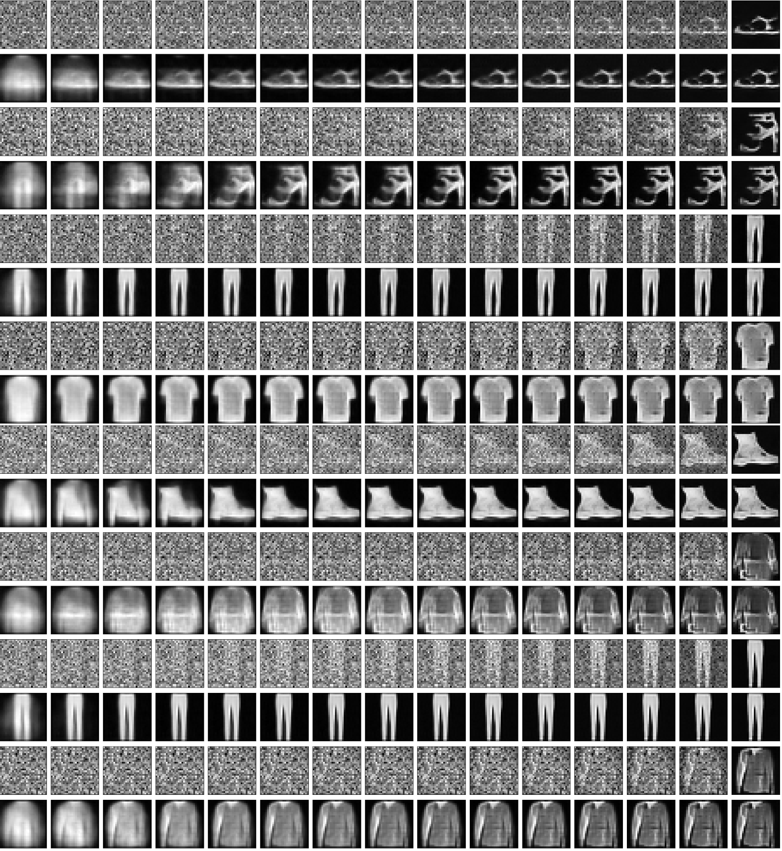
In Figure 3, we have shown some sampling results from the MNIST-Fashion dataset through the above sampling algorithm via building neural networks to estimate clean images.

II. Estimating noise \({\boldsymbol \epsilon}\)
In this case, we construct a deep neural network \(\boldsymbol \theta\) to approximate the inverse function via estimating the noise \({\boldsymbol \epsilon}\) from a corrupted image \(\mathbf{x}_t\) at each time step \(t\):
\[\hat{\boldsymbol \epsilon} = g^{-1}_{\boldsymbol \theta} (\mathbf{x}_t, t)\]This neural network is learned by minimizing the following objective function over all training data:
\[\begin{aligned} L_2({\boldsymbol \theta}) &= \sum_{\mathbf{x}_0 \in \mathcal{D}} \sum_{t=1}^T \Big( g^{-1}_{\boldsymbol \theta} (\mathbf{x}_t, t) - {\boldsymbol \epsilon}\Big)^2 \\ &= \sum_{\mathbf{x}_0 \in \mathcal{D}} \sum_{t=1}^T \Big( g^{-1}_{\boldsymbol \theta} \big(\sqrt{\bar{\alpha}_t} \mathbf{x}_{0} + \sqrt{1 - \bar{\alpha}_t} \, {\boldsymbol \epsilon}, t \big) - {\boldsymbol \epsilon}\Big)^2 \end{aligned}\]Once the neural network is learned, we can use Eq.(\ref{eq-consecutive-time-noise}) to derive an estimate of \(\mathbf{x}_{t-1}\) from \(\mathbf{x}_{t}\) as follows:
\[\begin{aligned} \mathbf{x}_{t-1} &= \frac{1}{\sqrt{\alpha_t}} \Big[ \mathbf{x}_t - \big( \sqrt{1-\bar{\alpha}_t} - \sqrt{\alpha_t-\bar{\alpha}_t} \big) \hat{\boldsymbol \epsilon} \Big] \\ &= \frac{1}{\sqrt{\alpha_t}} \Big[ \mathbf{x}_t - \big( \sqrt{1-\bar{\alpha}_t} - \sqrt{\alpha_t-\bar{\alpha}_t} \big) g^{-1}_{\boldsymbol \theta} (\mathbf{x}_t, t) \Big] \end{aligned}\]Similarly, the corresponding sampling process to generate a new image can be described as follows:
-
sample a Gaussian noise \(\mathbf{x}_T \sim \mathcal{N}(0, \mathbf{I})\)
-
for \(t=T, T-1, \cdots, 1\):
- use the trained neural network \({\boldsymbol \theta}\) to compute:
- estimate clean image as in Eq.(\ref{eq-forwar-t}):
-
if \(\hat{\mathbf{x}}_0\) is stable or \(t=1\), return \(\hat{\mathbf{x}}_0\)
-
else denoise one step backward as
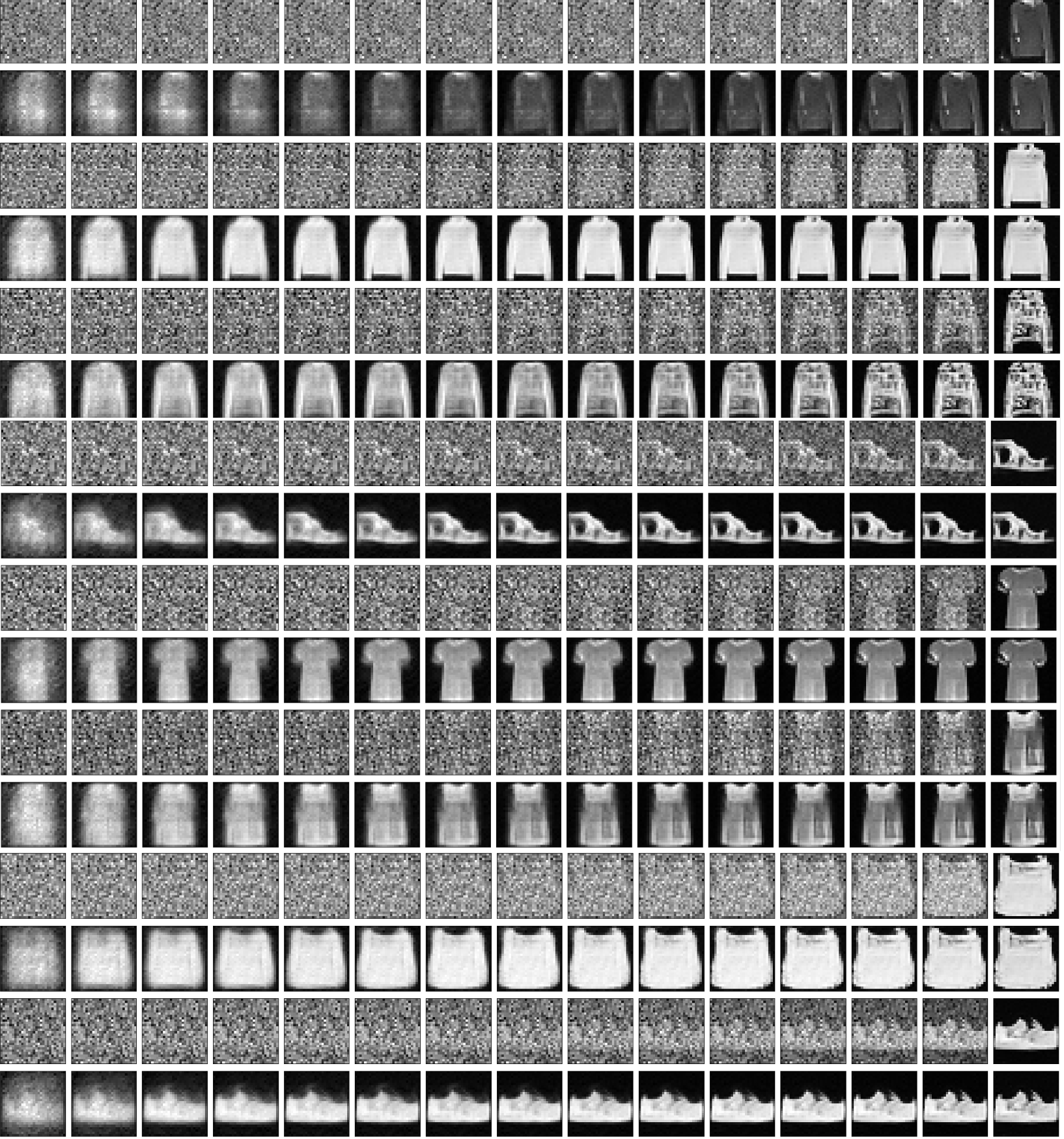
In Figure 4, we have shown some sampling results from the MNIST-Fashion dataset via building neural networks to estimate noises through the above sampling algorithm.

Final Remarks
In recent years, diffusion models have become increasingly significant in computer vision, emerging as the dominant models for images and videos across a wide range of real-world applications. However, the traditional approach to understanding diffusion models presents a steep learning curve, as it requires advanced mathematical knowledge in areas such as probability density estimation, stochastic process, and differential equation